 By far the most commonly used micromouse sensors are simple reflective types that give an indication of distance by measuring how much light is reflected from the maze wall. While the response is repeatable and related to distance, it is quite difficult to get an accurate answer. This is how the sensor readings can be converted into an actual distance…
This type of sensor has many limitations. The reading depends upon the angle between the emitter and the wall, the reflectivity of the wall itself and the geometry of the emitter and detector. For more experiments about the effect of the angle, look at this earlier post.
Typically, a narrow-beam Infra Red LED shines a spot of light onto the maze wall and a photodiode or phototransistor measures the light level. Two readings can be taken. The first is done with the emitter of and the second with the emitter on. The difference between the two readings should be due almost entirely to the effect of the emitter so that you can cancel out the effect of the ambient light. It is worth pointing out two problems with this technique, not related to the walls. First, the sensitivity of the detector will be affected by the ambient light level so you cannot entirely eliminate this. Second, the detector may be close to saturation with the emitter off as a result of high ambient light levels so that turning on the emitter does not produce a reading as high as it would be in the absence of ambient illumination.
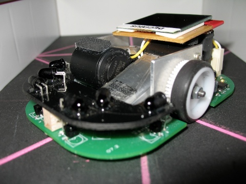
My mouse has six sensor assemblies. Two face almost sideways, two face diagonally at around 45 degrees to the direction of travel and two more face nearly forwards, in front of the mouse. To measure the response of these sensors, the mouse was place on a moving platform (the cross-slide of my lathe) and a wall arranged appropriately to the mouse axis in orientation seen by a correctly positioned mouse. Thus, for the forward sensor readings, the mouse faced the wall directly with the wall perpendicular to the long axis of the mouse. For the side and diagonal sensor tests, the wall was place parallel to the long axis of the mouse. Now the distance between the edge of the mouse and the wall can be changed accurately in fixed steps and readings taken from the sensors. I chose steps of 6mm to keep the volume of manually collected data manageable. The edge of the mouse is used for distance measurements rather than the centre of the mouse because this feels more practical. When the distance gets to zero, the mouse is in contact with the wall. the results for all six sensors can be seen in this chart:
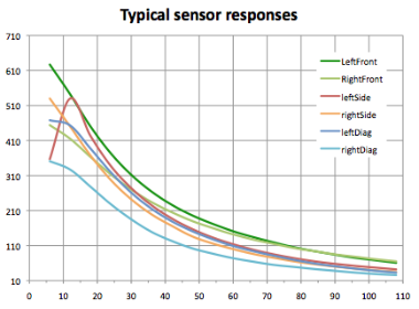 Here the raw ADC value is plotted against distance. You can see immediately that the reading is not linearly related to the distance although it is monotonic beyond about 15mm. That is, increasing the distance always makes the reading decrease. at distances of less than 15mm, the shape of the graph changes. Mostly, this is because the physical arrangement of the emitter-detector pair on my mouse means that the spot of light is not visible by the detector when the wall is very close. this is a design flaw that could be largely corrected. It does not generally cause any trouble because, by the time you are within 15mm of a wall, you are already in trouble and the exact distance is not terribly relevant. You should also notice that the forward sensors are less affected close to the wall. This is by design to make it more reliable when gauging distance to the wall ahead for aligning the mouse
The various sensors have different sized responses even though they were all very carefully aligned to specific geometries when the mouse was assembled. Manufacturing tolerances mean that, for the same current, each emitter will be a slightly different brightness and, for a given level of illumination, each detector will give a different response. While it would be possible to buy in large numbers of emitters and detectors and select matching pairs, that is not a practical, or economic solution.
What is reasonably clear, however, is that the shape of the graph for each sensor is very similar even though they have different orientations to the wall. If we suppose that each curve is determined by the same equation but with different constants, it should be possible to determine the appropriate constants for each sensor and convert the reading into a reliable measure of distance.
The question is – what equation would generate the shape that we see.
Excel lets you fit a trend line to the data but none of the available options gave a convincing fit. To cut a long story short, eventually I found a function that gave a very good fit to the data:
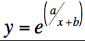 Where y is the sensor reading, x is the distance to the wall, and a and b are constants which will be different for each sensor and the reflectivity of the walls.
Taking the left front sensor data as an example, we can calculate that the appropriate values for a and b in the test setup are 1182 and 176 respectively. Plotting both the fitted and the original data on the same axes give us this result:
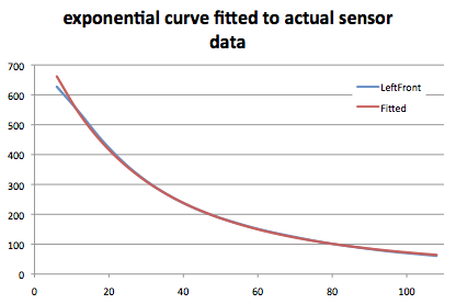 This fits the data so well that the variation can only be seen at very short distances where we know that other effects change the response of the sensor.
Now that it is possible to determine a function that fits the results, it can be manipulated so that, for a given sensor reading, the distance can be determined. Rearranging the equation above gives us:
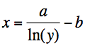 Again, y is the sensor reading and x is the distance. By now you will probably have thought of a couple of problems with this approach. First, how do you determine the constants a and b, and how much work will it be to calculate a natural logarithm and a divide for each sensor reading, bearing in mind that we want to do six of these every millisecond or so.
Taking the second problem first, I pre-calculated a table of natural logarithms for all values of 1 to 1023. Since I have a 10 bit ADC, this quickly allows me to look up the logarithm directly from the sensor reading. Inconveniently, logarithms are fractional values but that is easily fixed by pre-multiplying each by 65536 to give a 16.16 fixed point value in the table. If the constant a is also scaled by the same amount, the result of the division gives us an integer result. All we need worry about then is a 32 bit divide which is not overly burdensome on a fast processor like the dsPIC or STM32. If you have a slower processor, you will want to optimise that a bit more. For example, you could generate a 16 bit value with 12 bits for the fractional part and leave yourself with a 16 bit divide.
How well does it work? Well, here is a chart showing the calculated distance, in mm against the actual distances recorded from the raw data.
 The correspondence between the two is remarkably good and well within the various errors that are unavoidable with this type of sensor.
So, how to calculate the constants? The equation above has two unknowns, an and b. All we require are two sensor readings at known distances from the walls and a bit of gentle algebra will allow us to work those out. One of the sets of readings can be taken with the mouse placed as close as possible to the centre of a maze cell. using this as one of your fixed points ensures that the fitted curve will be that little bit more accurate at that distance. The other point is most conveniently having the mouse hard up against the far wall for each sensor. This is a known distance which, by the magic of geometry is easy to determine from the dimensions of your mouse. I will leave the task of figuring out how to calculate a and b as an exercise for the reader so that you feel that you have actively participated.
It may occur to you that there is a potential problem with this technique as the distances get larger. Since typical sensor readings at a distance of 100mm or so are down to, perhaps 60 out of a range of 1023, the effect of small changes in sensor reading is proportionately much larger. The method will be very reliable over the range 20-100mm and progressively less reliable beyond that. However, I have found good results at distances up to 150mm where typical sensor readings are down to about 35. Even then, a difference in sensor reading of just one bit changes the calculated distance by about 3mm. At that range, it is not a serious issue.
There are only a couple of occasions where long range sensing is important unless you are trying to map walls in adjacent cells without visiting them. When exploring, it is important to be able to detect a wall ahead as soon as you can. When the front of the mouse enters a cell, the far wall will be about 170mm away. It is easy to tell that a wall is there and the error in its measured position will be relatively large but, at this stage relatively unimportant. As the mouse wheels cross the threshold, the far wall will be a about 130mm away – well within reliable enough measurement range. Bear in mind that wall reflectivity plays a crucial role in this business and the walls I have – all Korean – show variations as great as 10% in the extreme so really accurate measurements using just reflective light are a bit of a pipe-dream anyway.
Another time you see apparently distant walls is when passing a lone post. if your emitter beam-width is large compared to the size of a post, the amount of light reflected is less that it would be from a section of wall at the same distance. Consequently, the post will appear to be a section of wall way off in the distance. You need to look out for that and compensate accordingly. On Decimus2, the most advantageously positioned sensors – the side-looking pair – see a lone post at an apparent distance of about 75mm while a wall would appear to be about 42mm away.
Addendum:
The chart below shows actual results from the mouse in part of the maze:
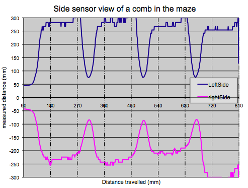 Here the mouse starts off in the middle of a cell with walls on either side and then runs down a short section with only perpendicular walls on either side – a comb. The side sensor results, converted to distance are plotted with the right side represented as a negative number. It is fairly clear that the posts generate a smaller response and that the calibration generates good results out to beyond a perceived 150mm. As the distance gets larger, the effects of quantisation on small sensor readings are also apparent. If there had been a parallel wall at the far side of the adjacent cell, it would have been about 240mm away from the mouse. At that distance, the response is down into the noise region and the sensors, as configured, would not be able to detect it. I cannot recall whether there were walls present for this trial.
With a similar emitter – sensor arrangement, initially had the sensor reading to distance conversion problem, but I just used a look-up table to give distance from the on/off ADC value difference.
But for the heading correction it appears unnecessary, just use the ADC on/off difference value: in the starting cell the side looking sensors should have equal value and this gives your rough calibration of the threshold value for steering correction: when lower than this move towards wall and when greater move away. Using a threshold to correct heading does sometimes seem to cause an oscillating path, so finer error (value) control might be an advantage.
As you noted, there are a few important distances, but since you are often just comparing to see if you are closer or not than a distance: instead of converting the changing ADC value to distance, convert the fixed distance to ADC value.
If you wish to use logs, using log 2 instead of natural might be easier: loga x = logb x / logb a
Yes, there is no need to go to all that trouble just to get the mouse to run straight. Also, you can store fixed values for critical distances so that is fine.
However, the question of how to reliably get a distance from the sensors has been bugging be for ages and, having found a method that seems to be robust, I just had to put it up.
Besides, if you can do the calibration, your code is free of magic numbers and can just use distances for critical values knowing that a simple sensor calibration sorts out all the values when you get to a new maze.
Im having trouble determining these constants, even though it was the only thing you left the readers to do for themselves! However, I’m wondering when you determine one constant from placing the mouse in the center of the maze if the distance should be measured or the ADC value will become the constant? Also, should the entire dimensions of the mouse be used? or just the dimensions of the IR sensor array we have.
Thanks!
I am no longer going to this much trouble to be honest. After a chat with Khiew Tzong Yong, I am taking his advice and calculating a single calibration constant.
The sensor response for walls of a different reflectivity is simply shifted up or down and the shape of the response remains the same. So, we get something like this:
where k is some constant you will need to determine for each sensor. Measure the intensity at the central position of the mouse and call this I’ then choose k such that the value for D is, say, 100 at this point. Recalibrating for a different wall just means finding a new value for k.
Thanks for the response!
So now I’m wondering if I is the ADC value and I’ is the ADC value tested. Also can the recalibration be done by the mouse programmatically for different reflectivities??
Pingback: Kalibracja czujnika ściany - ucgosu.pl